Note
Go to the end to download the full example code.
PyLossless Algorithms
This tutorial explains the calculations that PyLossless performs at each step of the pipeline. We will use example EEG data to demonstrate the calculations.
Note
You can open this notebook in Google Colab!
Notation
Before we begin, we define some notation that will be used throughout the text:
We start with a 3D matrix of EEG data, \(X \in \mathbb{R}^{S_\mathcal{G} \times E_\mathcal{G} \times T}\), where \(S_\mathcal{G}\) and \(E_\mathcal{G}\) are the sets of good sensors and epochs, respectively, and \(T\), is the number of samples(i.e. time-points).
s,e, andtare sensor, epochs, and samples, respectively.We use superscripts to denote operations across a dimension, and we use subscripts to denote indexing a dimension.
We refer to a single sensor \(i\) as \(X\big|_{s=i} \in \mathbb{R}^{E_\mathcal{G} \times T}\), with \(i \in S_\mathcal{G}\).
We refer to a single epoch \(j\) as \(X\big|_{e=j} \in \mathbb{R}^{S_\mathcal{G} \times T}\), with \(j \in E_\mathcal{G}\).
We denote sensor-specific thresholds for rejecting epochs as \(\tau^e_i \in \mathbb{R}^{S_\mathcal{G}}\)
We denote epoch-specific thresholds for rejecting sensors as \(\tau^s_j \in \mathbb{R}^{E_\mathcal{G}}\)
We denote quantiles as \(Q\#^{dim}\): i.e. \(Q75^s\) is the 75th quantile along the sensor dimension. The function \(Q75^s(X)\) computes the 75th quantile along the \(s\) dimension of matrix \(X\), resulting in a matrix noted \(X^{Q75^s} \in \mathbb{R}^{E \times T}\).
Throughout the text, we use capital letters for matrices and lowercase letters for scalars. For example, the data point for sensor \(i\), epoch \(j\), and time \(k\) is denoted as \(X\big|_{s=i; e=j; t=k} = x_{ijk} \in \mathbb{R}\), and \(X=\{x_{ijk}\}\).
Imports and data loading
from pathlib import Path

import numpy as np

import mne
from mne.datasets import sample

import pylossless as ll

# Load example mne data
raw = ll.datasets.load_simulated_raw()
Using default location ~/mne_data for sample...
Creating /home/docs/mne_data

  0%|                                              | 0.00/1.65G [00:00<?, ?B/s]
  0%|                                      | 254k/1.65G [00:00<10:59, 2.51MB/s]
  0%|                                     | 2.80M/1.65G [00:00<01:43, 15.9MB/s]
  1%|▎                                    | 13.7M/1.65G [00:00<00:28, 58.2MB/s]
  2%|▌                                    | 25.7M/1.65G [00:00<00:19, 82.6MB/s]
  2%|▊                                    | 37.8M/1.65G [00:00<00:16, 96.5MB/s]
  3%|█▏                                    | 49.5M/1.65G [00:00<00:15, 103MB/s]
  4%|█▍                                    | 60.2M/1.65G [00:00<00:15, 105MB/s]
  4%|█▋                                    | 73.2M/1.65G [00:00<00:14, 113MB/s]
  5%|█▉                                    | 84.4M/1.65G [00:00<00:14, 107MB/s]
  6%|██▏                                   | 97.2M/1.65G [00:01<00:13, 113MB/s]
  7%|██▌                                    | 109M/1.65G [00:01<00:14, 108MB/s]
  7%|██▊                                    | 120M/1.65G [00:01<00:13, 111MB/s]
  8%|███▏                                   | 133M/1.65G [00:01<00:13, 115MB/s]
  9%|███▍                                   | 144M/1.65G [00:01<00:13, 115MB/s]
  9%|███▋                                   | 157M/1.65G [00:01<00:12, 118MB/s]
 10%|███▉                                   | 169M/1.65G [00:01<00:12, 120MB/s]
 11%|████▎                                  | 181M/1.65G [00:01<00:12, 119MB/s]
 12%|████▌                                  | 193M/1.65G [00:01<00:12, 119MB/s]
 12%|████▊                                  | 205M/1.65G [00:01<00:12, 119MB/s]
 13%|█████                                  | 217M/1.65G [00:02<00:12, 119MB/s]
 14%|█████▍                                 | 229M/1.65G [00:02<00:11, 119MB/s]
 15%|█████▋                                 | 241M/1.65G [00:02<00:11, 119MB/s]
 15%|█████▉                                 | 253M/1.65G [00:02<00:11, 117MB/s]
 16%|██████▎                                | 265M/1.65G [00:02<00:11, 119MB/s]
 17%|██████▌                                | 277M/1.65G [00:02<00:11, 119MB/s]
 17%|██████▊                                | 289M/1.65G [00:02<00:11, 119MB/s]
 18%|███████                                | 301M/1.65G [00:02<00:11, 119MB/s]
 19%|███████▍                               | 313M/1.65G [00:02<00:11, 119MB/s]
 20%|███████▋                               | 325M/1.65G [00:02<00:11, 119MB/s]
 20%|███████▉                               | 337M/1.65G [00:03<00:11, 118MB/s]
 21%|████████▏                              | 349M/1.65G [00:03<00:10, 120MB/s]
 22%|████████▌                              | 361M/1.65G [00:03<00:10, 120MB/s]
 23%|████████▊                              | 373M/1.65G [00:03<00:10, 118MB/s]
 23%|█████████                              | 385M/1.65G [00:03<00:10, 118MB/s]
 24%|█████████▎                             | 397M/1.65G [00:03<00:10, 118MB/s]
 25%|█████████▋                             | 409M/1.65G [00:03<00:10, 118MB/s]
 25%|█████████▉                             | 421M/1.65G [00:03<00:10, 119MB/s]
 26%|██████████▏                            | 433M/1.65G [00:03<00:10, 119MB/s]
 27%|██████████▍                            | 445M/1.65G [00:03<00:10, 119MB/s]
 28%|██████████▊                            | 457M/1.65G [00:04<00:10, 119MB/s]
 28%|███████████                            | 469M/1.65G [00:04<00:09, 119MB/s]
 29%|███████████▎                           | 481M/1.65G [00:04<00:09, 118MB/s]
 30%|███████████▌                           | 492M/1.65G [00:04<00:09, 118MB/s]
 31%|███████████▉                           | 504M/1.65G [00:04<00:09, 119MB/s]
 31%|████████████▏                          | 516M/1.65G [00:04<00:09, 119MB/s]
 32%|████████████▍                          | 529M/1.65G [00:04<00:09, 120MB/s]
 33%|████████████▊                          | 541M/1.65G [00:04<00:09, 121MB/s]
 33%|█████████████                          | 553M/1.65G [00:04<00:09, 120MB/s]
 34%|█████████████▎                         | 565M/1.65G [00:04<00:09, 109MB/s]
 35%|█████████████▌                         | 576M/1.65G [00:05<00:10, 103MB/s]
 36%|█████████████▉                         | 589M/1.65G [00:05<00:09, 110MB/s]
 36%|██████████████▏                        | 602M/1.65G [00:05<00:09, 114MB/s]
 37%|██████████████▍                        | 614M/1.65G [00:05<00:08, 116MB/s]
 38%|██████████████▊                        | 626M/1.65G [00:05<00:08, 118MB/s]
 39%|███████████████                        | 638M/1.65G [00:05<00:08, 120MB/s]
 39%|███████████████▎                       | 651M/1.65G [00:05<00:08, 121MB/s]
 40%|███████████████▋                       | 663M/1.65G [00:05<00:08, 119MB/s]
 41%|███████████████▉                       | 675M/1.65G [00:05<00:08, 121MB/s]
 42%|████████████████▏                      | 688M/1.65G [00:06<00:07, 122MB/s]
 42%|████████████████▌                      | 700M/1.65G [00:06<00:07, 122MB/s]
 43%|████████████████▊                      | 712M/1.65G [00:06<00:07, 121MB/s]
 44%|█████████████████                      | 725M/1.65G [00:06<00:07, 121MB/s]
 45%|█████████████████▍                     | 737M/1.65G [00:06<00:07, 121MB/s]
 45%|█████████████████▋                     | 749M/1.65G [00:06<00:07, 121MB/s]
 46%|█████████████████▉                     | 761M/1.65G [00:06<00:07, 121MB/s]
 47%|██████████████████▎                    | 774M/1.65G [00:06<00:07, 123MB/s]
 48%|██████████████████▌                    | 786M/1.65G [00:06<00:07, 121MB/s]
 48%|██████████████████▊                    | 798M/1.65G [00:06<00:07, 121MB/s]
 49%|███████████████████▏                   | 811M/1.65G [00:07<00:06, 122MB/s]
 50%|███████████████████▍                   | 823M/1.65G [00:07<00:06, 122MB/s]
 51%|███████████████████▋                   | 835M/1.65G [00:07<00:06, 123MB/s]
 51%|███████████████████▉                   | 848M/1.65G [00:07<00:06, 122MB/s]
 52%|████████████████████▎                  | 860M/1.65G [00:07<00:06, 122MB/s]
 53%|████████████████████▌                  | 872M/1.65G [00:07<00:06, 122MB/s]
 54%|████████████████████▊                  | 884M/1.65G [00:07<00:06, 122MB/s]
 54%|█████████████████████▏                 | 897M/1.65G [00:07<00:06, 123MB/s]
 55%|█████████████████████▍                 | 909M/1.65G [00:07<00:06, 121MB/s]
 56%|█████████████████████▋                 | 921M/1.65G [00:07<00:06, 121MB/s]
 56%|██████████████████████                 | 933M/1.65G [00:08<00:05, 122MB/s]
 57%|██████████████████████▎                | 946M/1.65G [00:08<00:05, 123MB/s]
 58%|██████████████████████▌                | 958M/1.65G [00:08<00:05, 123MB/s]
 59%|██████████████████████▉                | 970M/1.65G [00:08<00:05, 122MB/s]
 59%|███████████████████████▏               | 983M/1.65G [00:08<00:05, 122MB/s]
 60%|███████████████████████▍               | 995M/1.65G [00:08<00:05, 122MB/s]
 61%|███████████████████████▏              | 1.01G/1.65G [00:08<00:05, 122MB/s]
 62%|███████████████████████▍              | 1.02G/1.65G [00:08<00:05, 122MB/s]
 62%|███████████████████████▋              | 1.03G/1.65G [00:08<00:05, 122MB/s]
 63%|████████████████████████              | 1.04G/1.65G [00:08<00:04, 122MB/s]
 64%|████████████████████████▎             | 1.06G/1.65G [00:09<00:04, 122MB/s]
 65%|████████████████████████▌             | 1.07G/1.65G [00:09<00:04, 122MB/s]
 65%|████████████████████████▊             | 1.08G/1.65G [00:09<00:04, 123MB/s]
 66%|█████████████████████████▏            | 1.09G/1.65G [00:09<00:04, 123MB/s]
 67%|█████████████████████████▍            | 1.11G/1.65G [00:09<00:04, 122MB/s]
 68%|█████████████████████████▋            | 1.12G/1.65G [00:09<00:04, 122MB/s]
 68%|█████████████████████████▉            | 1.13G/1.65G [00:09<00:04, 120MB/s]
 69%|██████████████████████████▎           | 1.14G/1.65G [00:09<00:04, 123MB/s]
 70%|██████████████████████████▌           | 1.16G/1.65G [00:09<00:04, 122MB/s]
 71%|██████████████████████████▊           | 1.17G/1.65G [00:09<00:03, 122MB/s]
 71%|███████████████████████████           | 1.18G/1.65G [00:10<00:03, 118MB/s]
 72%|███████████████████████████▍          | 1.19G/1.65G [00:10<00:04, 104MB/s]
 73%|███████████████████████████▋          | 1.20G/1.65G [00:10<00:04, 103MB/s]
 73%|███████████████████████████▉          | 1.21G/1.65G [00:10<00:04, 108MB/s]
 74%|████████████████████████████▏         | 1.23G/1.65G [00:10<00:03, 112MB/s]
 75%|████████████████████████████▍         | 1.24G/1.65G [00:10<00:03, 114MB/s]
 76%|████████████████████████████▊         | 1.25G/1.65G [00:10<00:03, 116MB/s]
 76%|█████████████████████████████         | 1.26G/1.65G [00:10<00:03, 118MB/s]
 77%|█████████████████████████████▎        | 1.28G/1.65G [00:10<00:03, 120MB/s]
 78%|█████████████████████████████▌        | 1.29G/1.65G [00:11<00:03, 121MB/s]
 79%|█████████████████████████████▉        | 1.30G/1.65G [00:11<00:02, 120MB/s]
 79%|██████████████████████████████▏       | 1.31G/1.65G [00:11<00:02, 121MB/s]
 80%|██████████████████████████████▍       | 1.32G/1.65G [00:11<00:02, 121MB/s]
 81%|██████████████████████████████▋       | 1.34G/1.65G [00:11<00:02, 121MB/s]
 82%|███████████████████████████████       | 1.35G/1.65G [00:11<00:02, 122MB/s]
 82%|███████████████████████████████▎      | 1.36G/1.65G [00:11<00:02, 105MB/s]
 83%|███████████████████████████████▌      | 1.37G/1.65G [00:11<00:02, 101MB/s]
 84%|███████████████████████████████▊      | 1.39G/1.65G [00:11<00:02, 109MB/s]
 85%|████████████████████████████████▏     | 1.40G/1.65G [00:12<00:02, 114MB/s]
 85%|████████████████████████████████▍     | 1.41G/1.65G [00:12<00:02, 116MB/s]
 86%|████████████████████████████████▋     | 1.42G/1.65G [00:12<00:02, 114MB/s]
 87%|████████████████████████████████▉     | 1.43G/1.65G [00:12<00:01, 113MB/s]
 87%|█████████████████████████████████▏    | 1.44G/1.65G [00:12<00:01, 109MB/s]
 88%|█████████████████████████████████▍    | 1.46G/1.65G [00:12<00:01, 113MB/s]
 89%|█████████████████████████████████▊    | 1.47G/1.65G [00:12<00:01, 115MB/s]
 90%|██████████████████████████████████    | 1.48G/1.65G [00:12<00:01, 117MB/s]
 90%|██████████████████████████████████▎   | 1.49G/1.65G [00:12<00:01, 119MB/s]
 91%|██████████████████████████████████▋   | 1.51G/1.65G [00:12<00:01, 120MB/s]
 92%|██████████████████████████████████▉   | 1.52G/1.65G [00:13<00:01, 120MB/s]
 93%|███████████████████████████████████▏  | 1.53G/1.65G [00:13<00:01, 120MB/s]
 93%|███████████████████████████████████▍  | 1.54G/1.65G [00:13<00:00, 120MB/s]
 94%|███████████████████████████████████▋  | 1.55G/1.65G [00:13<00:00, 121MB/s]
 95%|████████████████████████████████████  | 1.57G/1.65G [00:13<00:00, 122MB/s]
 96%|████████████████████████████████████▎ | 1.58G/1.65G [00:13<00:00, 121MB/s]
 96%|████████████████████████████████████▌ | 1.59G/1.65G [00:13<00:00, 121MB/s]
 97%|████████████████████████████████████▊ | 1.60G/1.65G [00:13<00:00, 122MB/s]
 98%|█████████████████████████████████████▏| 1.62G/1.65G [00:13<00:00, 122MB/s]
 99%|█████████████████████████████████████▍| 1.63G/1.65G [00:13<00:00, 122MB/s]
 99%|█████████████████████████████████████▋| 1.64G/1.65G [00:14<00:00, 123MB/s]
100%|█████████████████████████████████████▉| 1.65G/1.65G [00:14<00:00, 122MB/s]
  0%|                                              | 0.00/1.65G [00:00<?, ?B/s]
100%|█████████████████████████████████████| 1.65G/1.65G [00:00<00:00, 11.7TB/s]
Attempting to create new mne-python configuration file:
/home/docs/.mne/mne-python.json
Could not read the /home/docs/.mne/mne-python.json json file during the writing. Assuming it is empty. Got: Expecting value: line 1 column 1 (char 0)
Download complete in 52s (1576.2 MB)
Opening raw data file /home/docs/mne_data/MNE-sample-data/MEG/sample/sample_audvis_raw.fif...
    Read a total of 3 projection items:
        PCA-v1 (1 x 10²)  idle
        PCA-v2 (1 x 10²)  idle
        PCA-v3 (1 x 10²)  idle
    Range : 25800 ... 192599 =     42.956 ...   320.670 secs
Ready.
EEG channel type selected for re-referencing
Adding average EEG reference projection.
1 projection items deactivated
Reading forward solution from /home/docs/mne_data/MNE-sample-data/MEG/sample/sample_audvis-meg-eeg-oct-6-fwd.fif...
    Reading a source space...
    Computing patch statistics...
    Patch information added...
    Distance information added...
    [done]
    Reading a source space...
    Computing patch statistics...
    Patch information added...
    Distance information added...
    [done]
    2 source spaces read
    Desired named matrix (kind = 3523 (FIFF_MNE_FORWARD_SOLUTION_GRAD)) not available
    Read MEG forward solution (7498 sources, 306 channels, free orientations)
    Desired named matrix (kind = 3523 (FIFF_MNE_FORWARD_SOLUTION_GRAD)) not available
    Read EEG forward solution (7498 sources, 60 channels, free orientations)
    Forward solutions combined: MEG, EEG
    Source spaces transformed to the forward solution coordinate frame
Setting up raw simulation: 1 position, "cos2" interpolation
Event information stored on channel:              STI 014
    Interval 0.000–2.000 s
Setting up forward solutions
Computing gain matrix for transform #1/1
    Interval 0.000–2.000 s
    Interval 0.000–2.000 s
    Interval 0.000–2.000 s
    Interval 0.000–2.000 s
    Interval 0.000–2.000 s
    Interval 0.000–2.000 s
    Interval 0.000–2.000 s
    Interval 0.000–2.000 s
    Interval 0.000–2.000 s
    10 STC iterations provided
[done]
Adding noise to 366/376 channels (366 channels in cov)
Sphere                : origin at (0.0 0.0 0.0) mm
              radius  : 0.1 mm
Source location file  : dict()
Assuming input in millimeters
Assuming input in MRI coordinates

Positions (in meters) and orientations
1 sources
ecg simulated and trace not stored
Setting up forward solutions
Computing gain matrix for transform #1/1
Sphere                : origin at (0.0 0.0 0.0) mm
              radius  : 0.1 mm
Source location file  : dict()
Assuming input in millimeters
Assuming input in MRI coordinates

Positions (in meters) and orientations
2 sources
blink simulated and trace stored on channel:      EOG 061
Setting up forward solutions
Computing gain matrix for transform #1/1
Adding noise to 60/60 channels (60 channels in cov)
Adding noise to 2/2 channels (2 channels in cov)
Creating RawArray with float64 data, n_channels=60, n_times=12010
    Range : 0 ... 12009 =      0.000 ...    19.995 secs
Ready.
Load a PyLossless configuration file
Let’s load a PyLossless configuration file. This file contains the parameters that
will be used for each step of the pipeline. For example, the noisy_channels
section contains the parameters for the Flag Noisy Sensors step. We can modify
these parameters to change the behavior of the pipeline. For example, we can change
the percent of epochs that a sensor must be noisy for it to be flagged via the
flag_crit parameter.
config = ll.config.Config()
config.load_default()
config["noisy_channels"]["outliers_kwargs"]["lower"] = 0.25  # lower quantile
config["noisy_channels"]["outliers_kwargs"]["upper"] = 0.75  # upper quantile
config["noisy_channels"]["flag_crit"] = 0.30  # percent of epochs that a sensor must be noisy
config.save("test_config.yaml")
Create a pipeline instance
pipeline = ll.LosslessPipeline("test_config.yaml")
pipeline.raw = raw
raw.plot()

<MNEBrowseFigure size 800x800 with 4 Axes>
Input Data
First, we epoch the data to be used for subsequent steps. Let our 3D matrix below be defined as \(X \in \mathbb{R}^{S \times E \times T}\) where \(X\) is a matrix of real numbers and of dimension \(S\) sensors \(\times$ E\) epochs times T times.
🧹 Epoching..
Not setting metadata
19 matching events found
No baseline correction applied
0 projection items activated
Using data from preloaded Raw for 19 events and 601 original time points ...
0 bad epochs dropped
🔍 Detecting channels to leave out of reference.
EEG channel type selected for re-referencing
Applying a custom ('EEG',) reference.
Let’s convert our epochs object into a named xarray.DataArray object.
from pylossless.pipeline import epochs_to_xr

#
epochs_xr = epochs_to_xr(epochs, kind="ch")
epochs_xr  # 277 epochs, 50 sensors, 602 samples per epoch
Robust Average Reference
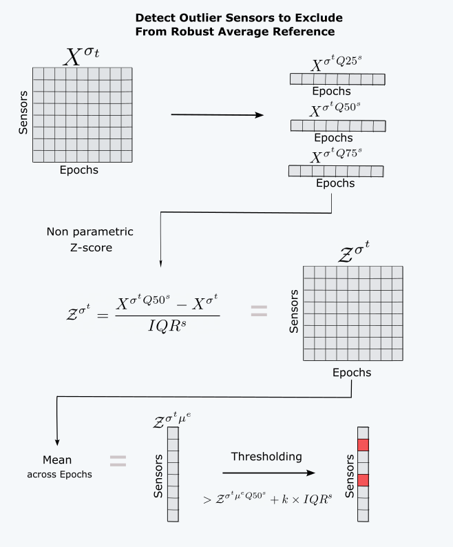
Robust Average Reference. The figure shows the steps for robust average referencing. See the text below for descriptions of mathematical notation.
Before the pipeline can begin, we must average reference the data. This is because the pipeline uses data distributions to identify noisy sensors, and For EEG data that uses an online reference to a single electrode, sensors that are further from the reference will have a higher voltage variance, and the pipeline will be biased to flag these sensors as noisy. The average reference, which subtracts the average signal across sensors from each individual sensor, will ensure an even playing field. Howeer, we dont want to include noisy sensors in the average reference signal. So we will identify noisy sensors and and leave them out of the average reference signal.
sample_std = epochs_xr.std("time")
q25_ch = sample_std.quantile(0.25, dim="ch")
q50_ch = sample_std.median(dim="ch")
q75_ch = sample_std.quantile(0.75, dim="ch")
ch_dist = sample_std - q50_ch  # center the data
ch_dist /= q75_ch - q25_ch  # shape (chans, epoch)

mean_ch_dist = ch_dist.mean(dim="epoch")  # shape (chans)

# find the median and 25 and 75 percentiles
# of the mean of the channel distributions
mdn = np.median(mean_ch_dist)
deviation = np.diff(np.quantile(mean_ch_dist, [0.25, 0.75]))

leave_out = mean_ch_dist.ch[mean_ch_dist > mdn + 6 * deviation].values.tolist()
leave_out
['EEG 001', 'EEG 002', 'EEG 007']
ref_chans = [ch for ch in epochs.pick("eeg").ch_names if ch not in leave_out]
pipeline.raw.set_eeg_reference(ref_channels=ref_chans)
EEG channel type selected for re-referencing
Applying a custom ('EEG',) reference.
Flag Noisy Sensors
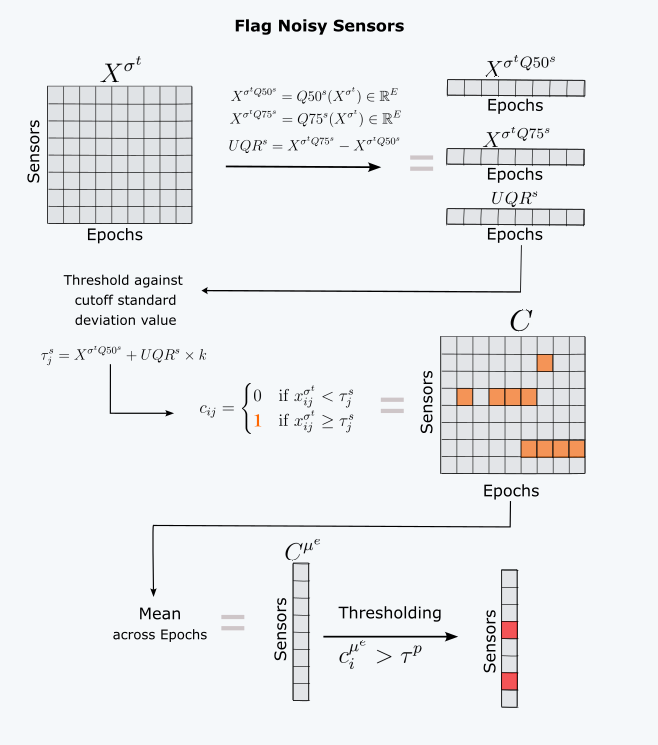
Flag Noisy Sensors. The figure shows the steps for flagging noisy sensors. See the text below for descriptions of mathematical notation.
Since we applied a robust average reference to the raw data, we will need to re-epoch the data:
epochs = pipeline.get_epochs()
epochs_xr = epochs_to_xr(epochs, kind="ch")

# First we take standard deviation of
# :math:`X \in \mathbb{R}^{S \times E \times T}` across the samples dimension :math:`t`
# resulting in a 2D matrix :math:`X^{\sigma_{t}} \in \mathbb{R}^{S \times E}`
trim_ch_sd = epochs_xr.std("time")
trim_ch_sd
🧹 Epoching..
Not setting metadata
19 matching events found
No baseline correction applied
0 projection items activated
Using data from preloaded Raw for 19 events and 601 original time points ...
0 bad epochs dropped
🔍 Detecting channels to leave out of reference.
EEG channel type selected for re-referencing
Applying a custom ('EEG',) reference.
a) Take the 50th and 75th quantile across dimension sensor of \(X^{\sigma_{t}}\)
This operation results in two 1D vectors of size \(E\):
q50, q75 = trim_ch_sd.quantile([0.5, 0.75], dim="ch")
q50  # a 1D array of median standard deviation values across channels for each epoch
b) Define an Upper Quantile Range as \(Q75 - Q50\)
This operation results in a 1D vector of size \(E\).
c) Identify outlier Indices \((i, j)\)
We multiply a constant \(k\) by the \(UQR\) to define a measure for the spread of the right tail of the distribution of \(X^{\sigma_{t}}\) values and add it to the median of \(X^{\sigma_{t}}\) to obtain epoch-specific standard deviation threshold for outliers:
That is, \(\tau^s_j\) is the epoch-specific threshold for the epoch \(j\)
k = 3
upper_threshold = q50 + q75 * k
upper_threshold  # epoch specific thresholds
Now, we compare our 2D standard deviation matrix to the threshold vector of \(\tau^e_j\):
resulting in the indicator matrix \(C \in \{0, 1\}^{S \times E}=\{c_{ij}\}\):
Each element of this matrix indicates whether sensor \(i\) is an outlier at an epoch \(j\).
d) Identify noisy sensors part 1
To identify outlier sensors, we average across the epoch dimension of our indicator matrix \(C\) and obtain \(C^{\mu_e} \in \mathbb{R}^{S_\mathcal{G}}\), which is a vector of fractional numbers \(c^{\mu_e}_i\) representing the percentage of epochs for which that sensor is an outlier.
percent_outliers = outlier_mask.astype(float).mean("epoch")
percent_outliers  # percent of epochs that sensor is an outlier
e) Identify noisy sensors part 2
Next, we define a threshold \(\tau^{p}\) (\(p\) for percentile;
default, .20) as a cutoff point for determining if a sensor should be marked
artifactual. The sensor \(i\) is flagged as noisy if
\(c^{\mu_e}_i > \tau^{p}\). That is, if the sensor is an outlier for more than
\(\tau^{p}\) percent of the epochs, it is flagged as noisy.
p_threshold = config["noisy_channels"]["flag_crit"]  # 0.3, or 30%
noisy_chs = percent_outliers[percent_outliers > p_threshold].coords.to_index().values
noisy_chs
array(['EEG 001', 'EEG 002'], dtype=object)
f) Add the noisy sensors to the pipeline flags
Let’s add the noisy sensors to the pipeline flags.
pipeline.flags["ch"].add_flag_cat(kind="noisy", bad_ch_names=noisy_chs)
pipeline.raw.info["bads"].extend(pipeline.flags["ch"]["noisy"].tolist())
pipeline.flags["ch"]
Flagged channels: |
  Noisy: ['EEG 001' 'EEG 002']
  Bridged: None
  Uncorrelated: None
  Rank: None
Flag Noisy Epochs
This step closely resembles the Flag Noisy Sensors step. For the sake of brevity we will be more concise in the documentation.
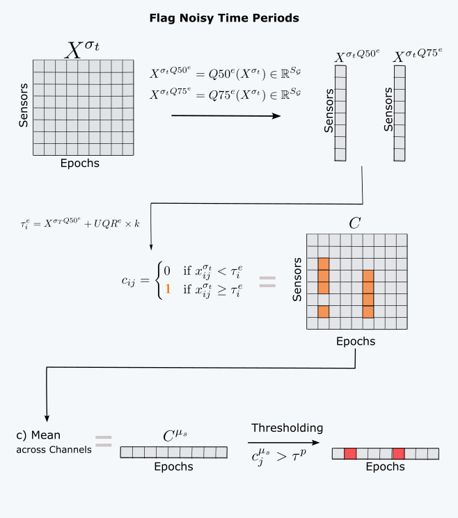
Flag Noisy Epochs. The figure shows the steps for flagging noisy epochs. See the text below for descriptions of mathematical notation.
a) Take standard deviation across the samples dimension \(t\)
Take a moment below to notice that the sensors flagged in the prior setp are not in
epochs_xr below:
epochs = pipeline.get_epochs()
# Let's make our epochs array into a named Array
epochs_xr = epochs_to_xr(epochs, kind="ch")
trim_ch_sd = epochs_xr.std("time")
trim_ch_sd.coords["ch"]
🧹 Epoching..
Not setting metadata
19 matching events found
No baseline correction applied
0 projection items activated
Using data from preloaded Raw for 19 events and 601 original time points ...
0 bad epochs dropped
🔍 Detecting channels to leave out of reference.
EEG channel type selected for re-referencing
Applying a custom ('EEG',) reference.
b) Compute 50th and 75th quantile across epochs and the UQR
Like before, We Take the median and 70th quantile, but now we operate across epochs,
resulting in two 1D vector’s of size n_good_sensors \(S_\mathcal{G}\)
c) Define sensor-specific thresholds for rejecting epochs \(\tau^e_i\)
Our sensor-specifc threshold for rejecting epochs is defined by:
k = 8
upper_threshold = q50 + uqr_epoch * k
upper_threshold
d) Identify Outlier indices
The indicator matrix is defined by:
To identify outlier epochs, we average across the sensor dimension of our indicator matrix \(C\) and obtain \(C^{\mu_s} \in \mathbb{R}^{E_\mathcal{G}}\), which is a vector of numbers \(c^{\mu_s}_j\) representing the percentage of sensors for which that epoch is an outlier.
percent_outliers = outlier_mask.astype(float).mean("ch")
percent_outliers
e) Identify noisy epochs
Next, we define a fractional threshold \(\tau^{p}\) as a cutoff point for determining if a epoch should be marked artifactual. The epoch \(j\) is flagged as noisy if \(c^{\mu_s}_j > \tau^{p}\).
bad_epochs = percent_outliers[percent_outliers > p_threshold].coords.to_index().values
bad_epochs
array([2])
f) Add the noisy epochs to the pipeline flags
Let’s add the outlier epochs to our flags
These will be added directly as mne.Annotations to the raw data.
pipeline.flags["epoch"].add_flag_cat(
    kind="noisy", bad_epoch_inds=bad_epochs, epochs=epochs
)
pipeline.raw.annotations.description
📋 LOSSLESS: 1.0 second(s) flagged as BAD_LL_noisy

array(['BAD_LL_noisy'], dtype='<U12')

<MNEBrowseFigure size 800x800 with 4 Axes>
Filtering
After flagging noisy sensors and epochs, we filter the data. By default, The pipeline uses a 1-100Hz bandpass filter. This is because 1), ICA decompositions are more stable when low frequency drifts are removed, and 2) the ICLabel classifier is trained on data that has been filtered between 1-100Hz. A notch filter can also be optionally specified.
pipeline.config["filtering"]["notch_filter_args"]["freqs"] = [50]
pipeline.filter()
LOSSLESS: 👇 filter.
Filtering raw data in 1 contiguous segment
Setting up band-pass filter from 1 - 1e+02 Hz

FIR filter parameters
---------------------
Designing a one-pass, zero-phase, non-causal bandpass filter:
- Windowed time-domain design (firwin) method
- Hamming window with 0.0194 passband ripple and 53 dB stopband attenuation
- Lower passband edge: 1.00
- Lower transition bandwidth: 1.00 Hz (-6 dB cutoff frequency: 0.50 Hz)
- Upper passband edge: 100.00 Hz
- Upper transition bandwidth: 25.00 Hz (-6 dB cutoff frequency: 112.50 Hz)
- Filter length: 1983 samples (3.302 s)

Filtering raw data in 1 contiguous segment
Setting up band-stop filter from 49 - 51 Hz

FIR filter parameters
---------------------
Designing a one-pass, zero-phase, non-causal bandstop filter:
- Windowed time-domain design (firwin) method
- Hamming window with 0.0194 passband ripple and 53 dB stopband attenuation
- Lower passband edge: 49.38
- Lower transition bandwidth: 0.50 Hz (-6 dB cutoff frequency: 49.12 Hz)
- Upper passband edge: 50.62 Hz
- Upper transition bandwidth: 0.50 Hz (-6 dB cutoff frequency: 50.88 Hz)
- Filter length: 3965 samples (6.602 s)

LOSSLESS: 🏁 Finished filter after 0.06 seconds.
Find Nearest Neighbours & return Maximum Correlation
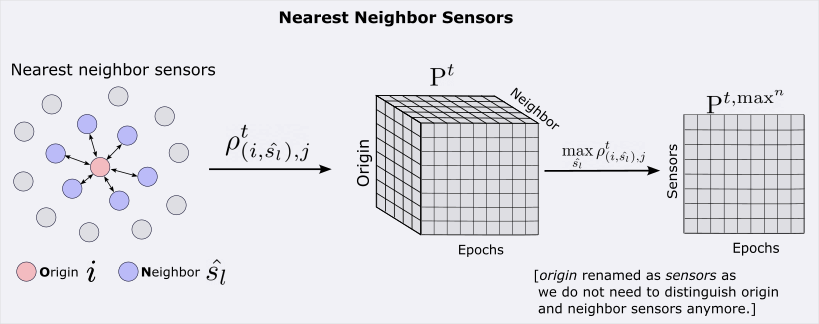
Nearest Neighbors. The figure shows the steps for finding nearest neighbors. See the text below for descriptions of mathematical notation.
Whereas Flag Noisy Sensors and Flag Noisy Epochs operated on a 2D matrix of standard deviation values, The next few steps will operate on correlation coefficients. Here we describe the procedure for defining the 2D matrix of correlation coefficients.
from pylossless.pipeline import chan_neighbour_r
Notice that our flagged epochs are dropped.
🧹 Epoching..
Not setting metadata
19 matching events found
No baseline correction applied
0 projection items activated
Using data from preloaded Raw for 19 events and 601 original time points ...
2 bad epochs dropped
🔍 Detecting channels to leave out of reference.
EEG channel type selected for re-referencing
Applying a custom ('EEG',) reference.
a) Calculate Correlation Coefficients between each Sensor and its neighboring eighbors
For each good sensor $i$ in \(S_{\mathcal{G}}\), we select its \(N\) nearest neighbors. I.e. the \(N\) sensors that are closest to it.
We call the sensor \(i\) the origin, and its nearest neighbors :math`hat{s_l}` with \(l \in \{1, 2, \ldots, N\}\)
Then, for each epoch \(j\), we calculate the correlation coefficient \(\rho^t_{(i,\hat{s_l}),j}\) between origin sensor \(i\) and each neighbor \(\hat{s_l}\) across dimension \(t\) (samples), returning a 3D matrice of correlation coefficients:
Finally, we select the maximum correlation coefficient across the neighbor dimension \(n\):
Returning a 2D matrix where each value at \((i, j)\) is the maximum correlation coefficient between sensor \(i\) and its \(N\) nearest neighbors, at each epoch \(j\)
data_r_ch = chan_neighbour_r(epochs, nneigbr=3, method="max")
# maximum correlation out of correlations between ch and its 3 neighbors
data_r_ch
  0%|          | 0/58 [00:00<?, ?it/s]
 14%|█▍        | 8/58 [00:00<00:00, 72.61it/s]
 28%|██▊       | 16/58 [00:00<00:00, 72.72it/s]
 41%|████▏     | 24/58 [00:00<00:00, 72.74it/s]
 55%|█████▌    | 32/58 [00:00<00:00, 73.00it/s]
 69%|██████▉   | 40/58 [00:00<00:00, 72.50it/s]
 83%|████████▎ | 48/58 [00:00<00:00, 72.49it/s]
 97%|█████████▋| 56/58 [00:00<00:00, 72.71it/s]
100%|██████████| 58/58 [00:00<00:00, 72.69it/s]
This matrix \(\mathrm{P}^{t,{\text{max}}^n}\) will be used in the steps below.
Flag Bridged Sensors
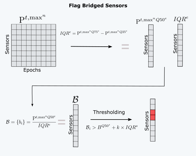
Flag Bridged Sensors. The figure shows the steps for flagging bridged sensors. See the text below for descriptions of mathematical notation.
a) Calculate the 50th, 75th quantile and IQR across epochs
For each sensor, divide the median across epochs by the IQR across epochs. Bridged channels should have a high median correlation but a low IQR of the correlation. We call this measure the bridge-indicator.
b) Define a bridging threshold
Now, take the 25th, 50th, and 75th quantile of \(\mathcal{B}_s\) across sensors, And calculate the \(IQR^s\). A channel \(i\) is bridged if
import scipy
from functools import partial
msr = data_r_ch.median("epoch") / data_r_ch.reduce(scipy.stats.iqr, dim="epoch")
# msr is a 1D vector of size n_sensors
config_trim = 40
config_bridge_z = 6
#
trim = config_trim
if trim >= 1:
    trim /= 100
trim /= 2  # .20 and will be used as (.20, .20)
#
trim_mean = partial(scipy.stats.mstats.trimmed_mean, limits=(trim, trim))
trim_std = partial(scipy.stats.mstats.trimmed_std, limits=(trim, trim))
#
z_val = config_bridge_z  # 6
mask = msr > msr.reduce(trim_mean, dim="ch") + z_val * msr.reduce(
    trim_std, dim="ch"
)  # bridged chans
#
bridged_ch_names = data_r_ch.ch.values[mask]
bridged_ch_names
array(['EEG 048', 'EEG 053', 'EEG 054'], dtype='<U7')
Let’s add the outlier channels to our flags
bad_chs = bridged_ch_names
pipeline.flags["ch"].add_flag_cat(kind="bridged", bad_ch_names=bad_chs)
pipeline.flags["ch"]
Flagged channels: |
  Noisy: ['EEG 001' 'EEG 002']
  Bridged: ['EEG 048' 'EEG 053' 'EEG 054']
  Uncorrelated: None
  Rank: None
Identify the Rank Channel
Because the pipeline uses an average reference before the ICA decomposition, it is necessary to account for rank deficiency (i.e., every sensor in the montage is linearly dependent on the other channels due to the common average reference). To account for this, the pipeline flags the sensor (out of the remaining good sensors) with the highest median of the max correlation coefficient with its neighbors (across epochs):
This sensor has the least unique time-series out of the remaining set of good sensors
\(S_\mathcal{G}\) and is flagged by the pipeline as ”rank”. Note that this
sensor is not flagged because it contains artifact, but only because one of the
remaining sensors needs to be removed to address rank deficiency before ICA
decomposition is performed. By choosing this sensor, we are likely to lose little
information because of its high correlation with its neighbors. This sensor can be
reintroduced after the ICA has been applied for artifact corrections.
good_chs = [
    ch for ch in data_r_ch.ch.values if ch not in pipeline.flags["ch"].get_flagged()
]
data_r_ch_good = data_r_ch.sel(ch=good_chs)

flag_ch = [str(data_r_ch_good.median("epoch").idxmax(dim="ch").to_numpy())]
pipeline.flags["ch"].add_flag_cat(kind="rank", bad_ch_names=flag_ch)
pipeline.flags["ch"]
Flagged channels: |
  Noisy: ['EEG 001' 'EEG 002']
  Bridged: ['EEG 048' 'EEG 053' 'EEG 054']
  Uncorrelated: None
  Rank: ['EEG 012']
Flag low correlation Epochs
This step is designed to identify time periods in which many sensors are uncorrelated with neighboring sensors. It is similar to the Flag Noisy Sensors step,
Again we calculate the 25th and 50th quantile of \(\mathrm{P}^{t,{\text{max}}^n}\), across the epochs dimension, and calculate the lower quantile range \(LQR^s\). This results in vectors \(\mathrm{P}^{t,{\text{max}}^nQ25^e}\) and \(\mathrm{P}^{t,{\text{max}}^nQ50^e}\) of size \(S_\mathcal{G}\). As for previous steps, we define sensor-specific thresholds for flagging epochs:
And the corresponding indicator matrix:
We average the indicator matrix across sensors and obtain a vector \(C^{\mu_s}\) that we use to flag uncorrelated epochs using the following criterion:
Step a
q25, q50 = data_r_ch.quantile([0.25, 0.5], dim="epoch")
#
# Define the LQR
lqr = q50 - q25
#
# define a threshold
k = 3
lower_threshold = q50 - lqr * k
#
outlier_mask = data_r_ch < lower_threshold
#
percent_outliers = outlier_mask.astype(float).mean("ch")
#
p_threshold = 0.2
bad_epochs = percent_outliers[percent_outliers > p_threshold].coords.to_index().values
#
# Add the outlier epochs to our flags
pipeline.flags["epoch"].add_flag_cat(
    kind="uncorrelated", bad_epoch_inds=bad_epochs, epochs=epochs
)
pipeline.raw.annotations.description
array(['BAD_LL_noisy'], dtype='<U12')
in this case, no epochs were flagged as uncorrelated.
Flag low correlation Sensors
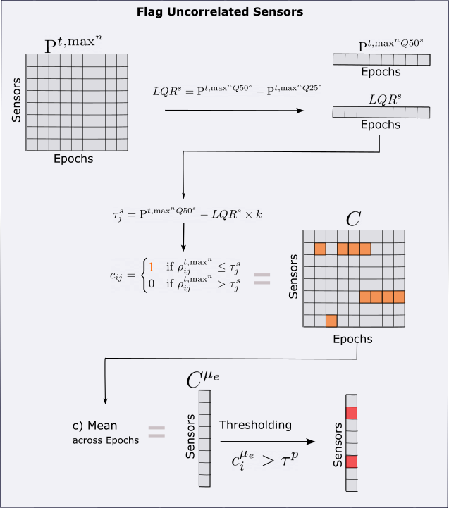
Flag Uncorrelated Sensors. The figure shows the steps for flagging uncorrelated sensors. See the text below for descriptions of mathematical notation.
This step is designed to identify sensors that have an unusually low correlation with neighboring sensors. The operations involved by this step are similar to those of the Flag Noisy Sensors step, except we use maximal nearest neighbor correlations instead of dispersion and the left instead of the right tail of the distribution to set the threshold for outliers.
a) Take lower quantile range and defined sensor-specific thresholds
We get the indicator matrix as described previously, using
and
Run Initial ICA
The pipeline by runs ICA two times. The first ICA is only used to identify noisy periods in its IC activation time-series. For this reason, the pipeline uses the FastICA algorithm for speed.
pipeline.run_ica("run1")
LOSSLESS: 👇 run_ica.
🧹 Epoching..
Not setting metadata
19 matching events found
No baseline correction applied
0 projection items activated
Using data from preloaded Raw for 19 events and 601 original time points ...
2 bad epochs dropped
🔍 Detecting channels to leave out of reference.
EEG channel type selected for re-referencing
Applying a custom ('EEG',) reference.
Fitting ICA to data using 54 channels (please be patient, this may take a while)
Selecting by non-zero PCA components: 53 components
/home/docs/checkouts/readthedocs.org/user_builds/pylossless/envs/latest/lib/python3.10/site-packages/sklearn/decomposition/_fastica.py:127: ConvergenceWarning: FastICA did not converge. Consider increasing tolerance or the maximum number of iterations.
  warnings.warn(
Fitting ICA took 5.2s.
LOSSLESS: 🏁 Finished run_ica after 5.31 seconds.
Flag Noisy IC Activation time-periods
This step follows the same procedure as the Flag Noisy Sensors step, except that the data is now the IC activation time-series. thus we start with a 3D matrix \(X_{ica} \in \mathbb{R}^{I_\mathcal{G} \times E_\mathcal{G} \times T}\) of IC time-courses rather than scalp EEG data and where \(I\) is the set of independent components.
LOSSLESS: 👇 flag_noisy_ics.
🧹 Epoching..
Not setting metadata
19 matching events found
No baseline correction applied
0 projection items activated
Using data from preloaded Raw for 19 events and 601 original time points ...
2 bad epochs dropped
🔍 Detecting channels to leave out of reference.
EEG channel type selected for re-referencing
Applying a custom ('EEG',) reference.
LOSSLESS: 🏁 Finished flag_noisy_ics after 0.14 seconds.
array(['BAD_LL_noisy'], dtype='<U12')
Run Final ICA
Now The pipeline runs the final ICA decomposition, this time using the extended Infomax algorithm. Note that any sensors or time-periods that have been flagged up to this point will not be passed into the ICA decomposition. For the sake of time, we will not run the second ICA here, as there are no more pipeline calculations.
Run ICLabel Classifier
The pipeline will run the ICLabel classifier on the final ICA, which will produce a
label for each IC, one of "brain", "muscle", "eog" (eye), "ecg"
(heart), line_noise, or "channel_noise".
Conclusion
And that’s all! See the other pylossless tutorials for brief examples on running the pipeline on your own data, and rejecting the flagged data.
Total running time of the script: (1 minutes 1.237 seconds)